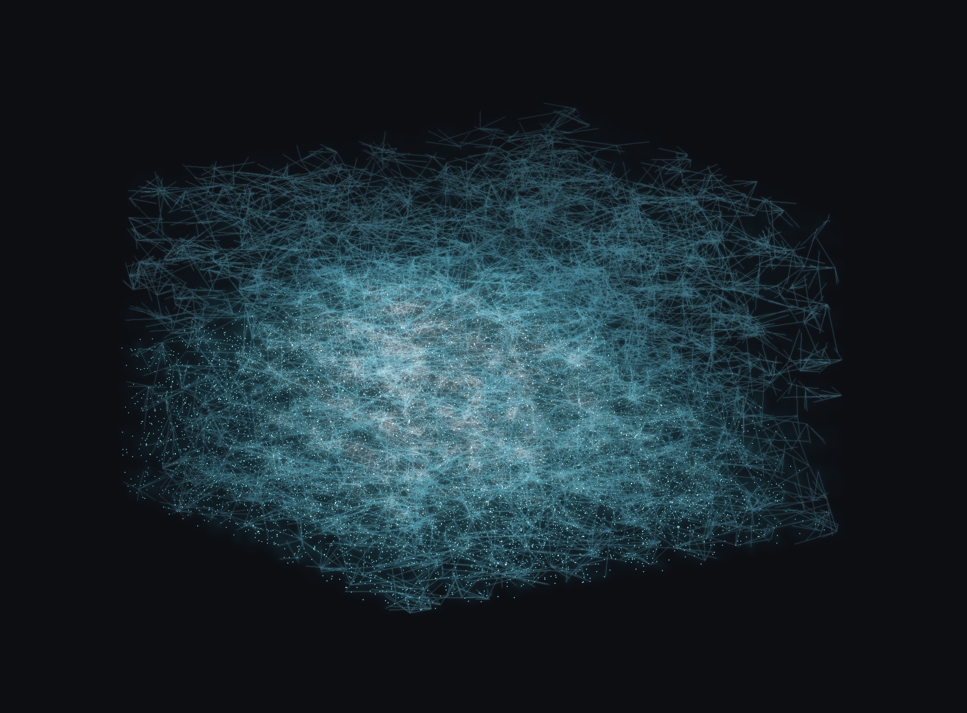
The essay describes a mind whose memory is a plastic graph — the terrain that thinking moves through. The figure is not a drawing of that idea; it is a real one. Two hundred thousand model neurons were placed in a cubic millimetre of simulated cortex, wired into a network, and left to fire on their own for twenty seconds of biological time, on a graphics card under a desk. What you see is that network and its measured activity. This page is exactly how it was built, and exactly where the honesty stops.
Step one
The engine: a living cell on a desktop GPU
The source is a small, single-purpose CUDA program — the first phase of a “volumetric brain engine,” whose only job is to answer one question honestly: does a truly three-dimensional spiking network come alive on its own, hold itself at the edge, and can we measure it? No task, no chatbot, no usefulness — just neurons, wiring, and physics. It runs far past real time at this scale on an ordinary RTX card, in about a third of a gigabyte of memory. Everything below is that program’s real output.
Step two
The wiring: structure is the prior
A brain is not a bag of neurons; it is a shape. The 200,000 cells are placed as a hierarchical-modular structure — clustered into 8×8×8 columns nested inside 2×2×2 areas — and then wired by a two-factor rule: a pair of neurons connects more readily the closer they sit and the more they share a module.
# wire each neuron to nearby cells, ~100 outgoing edges each:
P(i → j)  ∝  exp(−distance / λ)  ×  module_bias(i, j)

# λ = 150 µm  ·  same column ×1.0  ·  same area ×0.30  ·  different area ×0.06
That single rule builds a connectome of about twenty million synapses (a hundred out of each neuron), overwhelmingly local — 71% of edges stay inside a column, 28% within an area, and barely 1% reach across the whole volume. The result has a measured modularity of Q = 0.707: clustered and hierarchical, the way real cortex is, not a uniform random mesh. The glowing web in the figure is this wiring — the terrain, before anything fires.
Step three
The firing: spikes ride the edges
Each neuron is a compact Izhikevich spiking cell — a two-variable model that produces real spikes, not a rate. Eighty percent are excitatory, twenty inhibitory, as in cortex. Every tenth of a millisecond the whole network integrates, and whichever cells cross threshold fire; their spikes then ride the wiring — travelling along the edges, with an axonal delay, into the cells downstream.
# one tick = 0.1 ms of biological time:
integrate()          # Izhikevich v, u; cells over threshold spike
scatter_along_edges()# spikes follow the CSR wiring into a delay ring
homeostasis()        # two controllers hold it at the edge of alive
Left alone, such a network either falls silent or seizes. What keeps it alive is a pair of homeostatic controllers on separate timescales — a fast one that balances excitation against inhibition, a slow one that trims each cell’s input gain — plus a faint Poisson “breath” of background input so it never fully dies. Run for the full twenty seconds, the network self-sustains, and every neuron’s mean firing rate is written out. Those rates are the colours in the figure; the brightest points are the cells that fired hardest.
Step four
The honest part: alive is not the same as critical
The engine exists to be measured, not admired, and it is held to a real acceptance battery: is the network self-sustaining, is its branching ratio near one, are its cascades scale-free with the right exponents. This particular run is unmistakably alive — it breathes in great population avalanches (the largest swept over five million spikes) separated by quiet lulls, exactly the intermittent life the design is chasing.
But alive and cleanly critical are different claims, and the honest verdict is that whether this run sits at true criticality — rather than an intermittent regime that only resembles it — is still open. So the figure’s caption says exactly what is earned and no more: a modular connectome, firing. Never “a brain at criticality.” In the engine’s own words: failure of the gate is information, not defeat.
Step five
The render: the real data, in the essay's light
The picture is then built from the run’s actual output — the file of 200,000 positions and firing rates — in three honest layers, in the essay’s own void-and-cyan:
x, y, z, rate = load("neurons.csv")     # the real 200k positions + rates
field = smooth_volume(x, y, z, rate)    # the luminous body of the network
edges = rewire(x, y, z)                  # the connectome web (same rule, redrawn)
nodes = brightest(rate)                  # the hottest neurons, as vertices
One honest note about the web: the simulator keeps its full twenty-million-edge wiring in memory but never writes it to disk, so the figure re-draws a legible few-thousand-edge sample using the identical two-factor rule on the real neuron positions. It is representative wiring — the same statistics, the same locality and modularity — not the exact edge list. The positions and the firing rates are the true simulation output; the visible web is that output’s own rule, made visible.
What is real, and what is representative. Real: the 200,000 neuron positions, the modular structure, the firing rates, all straight from a live 20-second run. Representative: the drawn edges (the model’s own wiring rule re-applied to the real positions, since the exact list is never dumped). Unclaimed: criticality (the run is alive, not provably critical) and, exactly as in the essay, anything about whether there is something it is like to be it. The structure is real and the firing is real; the honesty is that the caption claims nothing more.
Reproduce it
Wire it, fire it, render it
The engine is a single CUDA build; the render is one Python script over the file it produces. Fixed seed, so the same connectome and the same firing come back every time.
# wire 200k neurons, run 20 s, write positions + rates
brain_phase0.exe            # -> neurons.csv, activity.csv
python tools/analyze.py     # the criticality battery, honest verdict

# render the real run in the essay's palette
python brain_render.py      # -> the connectome, firing